- Win rate measures only whether your favored side happened; it ignores the probability you assigned, so a 51%-calibrated forecaster and an overconfident 95% forecaster can post identical win rates while having wildly different forecasting skill.
- The Brier score is the mean squared error between stated probabilities and binary outcomes: BS = (1/N) Sum (f_t - o_t)^2. It ranges 0 (perfect) to 1 (worst), with 0.25 being the score of a 'fence-sitter' who always says 50%.
- Brier is a strictly proper scoring rule (Gneiting & Raftery, 2007): your expected score is best only when you report your true probability, so it cannot be gamed by hedging or exaggerating.
- The Murphy decomposition splits Brier into reliability (calibration), resolution (discrimination), and uncertainty — letting you separate 'are my probabilities honest?' from 'do I distinguish likely from unlikely events?'
- Log loss is the main alternative; it is unbounded and punishes confident errors far more harshly (a probability of 0 on an event that occurs is infinitely penalized), which is stricter but numerically fragile.
- Calibration evidence is why markets are taken seriously: the Iowa Electronic Markets beat polls in long-run studies, while a 2025 Vanderbilt study graded 2024 election markets with Brier and log loss and found wide accuracy gaps — proof these metrics, not win rate, are the standard.
The short answer
Win rate tells you how often the side you favored actually happened. It says nothing about whether your stated probabilities were right. A forecaster who calls every market at 51% and a reckless one who calls everything at 99% can post the identical win rate, yet only one of them is telling you the truth about uncertainty. Probabilistic forecasts need a probabilistic metric.
The Brier score is that metric. It is the mean squared error between the probability you assigned and the binary outcome (1 if the event happened, 0 if not), proposed by meteorologist Glenn W. Brier in 1950 (Monthly Weather Review). It rewards being calibrated — saying 70% when things happen 70% of the time — not just picking winners. Crucially, it is a strictly proper scoring rule: you minimize your expected score only by reporting your honest probability (Gneiting & Raftery, 2007). That is exactly the property a prediction-market trader, or a forecasting model, should be graded on.
Risk note: Event contracts and prediction markets carry real risk of loss. Nothing here is financial advice. Scoring metrics measure forecast quality, not profitability.
Calibration vs. accuracy: two different questions
These words get used interchangeably, and that confusion is the root of the problem.
- Accuracy / win rate asks: Did the outcome land on the side I leaned toward? It treats a forecast as a yes/no call. A 55% call and a 95% call both “win” if the event happens.
- Calibration asks: Across all the times I said X%, did the event happen X% of the time? A perfectly calibrated forecaster who says “70%” sees that event occur in roughly 70 of every 100 such cases — no more, no less.
Calibration is a property of the joint distribution of your predictions and outcomes, not of any single call (scikit-learn docs). A weather forecaster who says “30% chance of rain” and is correct that it rains on 30% of such days is perfectly calibrated, even though it didn’t rain most of the time. By win-rate logic, you might “mark them wrong” every dry day. That logic is broken for anything probabilistic.
There is a second, distinct virtue: resolution (also called discrimination or sharpness) — the ability to push probabilities away from the base rate toward 0 or 1 when you actually know something. A forecaster who says 50% on everything is perfectly calibrated in the long run but useless. Good scoring has to reward both honesty (calibration) and informativeness (resolution). The Brier score does.
Why win rate is misleading for probabilistic forecasts
Consider three traders forecasting the same ten binary markets. All three “win” the same number of markets — say, seven of ten by the majority-side test — so their win rates are identical at 70%. But watch what happens to their probability quality:
| Trader | Style | Typical probability on eventual winners | Win rate | Calibrated? |
|---|---|---|---|---|
| A | Honest | ~0.70 | 70% | Yes — events happen ~70% of the time |
| B | Overconfident | ~0.97 | 70% | No — claims near-certainty, wrong 30% of the time |
| C | Timid | ~0.55 | 70% | No — knows more than they admit |
Win rate cannot tell these three apart. Yet Trader B is dangerous — a 97% claim that fails 30% of the time signals badly miscalibrated risk — and Trader C is leaving information (and edge) on the table. The Brier score does separate them, because squaring the error punishes confident misses (B) and rewards confident-but-correct sharpness while penalizing needless timidity (C). This is why every serious forecasting tournament, from meteorology to geopolitics, abandoned raw accuracy decades ago.
There is also the simpler failure: on lopsided questions, “always predict the favorite” can post a glittering win rate while contributing zero forecasting skill. If 90% of your markets resolve in the favored direction, calling the favorite every time yields a 90% win rate and tells you nothing. Brier scores that strategy against the actual probabilities and exposes the hollowness.
The Brier score, defined
For binary outcomes, the Brier score is:
BS = (1/N) Σ (f_t − o_t)²
where f_t is the probability you assigned to event t (between 0 and 1), o_t is the outcome (1 if it happened, 0 if not), and N is the number of forecasts (Wikipedia). It is simply the mean squared error on probabilities.
Key properties:
- Range 0 to 1 in this modern binary form. 0 is perfect; 1 is the worst possible (you said 1.00 and it didn’t happen, every time). Brier’s original 1950 formulation ran 0 to 2; the binary version most people now use is exactly half of it (Wikipedia).
- 0.25 is the “fence-sitter” baseline. Assign 0.5 to everything and every squared error is 0.5² = 0.25, so your Brier score is exactly 0.25 (UVA Library). Any honest forecaster with real information should beat 0.25; a score above it means you are worse than a coin.
- Lower is better — it behaves like a golf score.
- It is a strictly proper scoring rule, so the only way to minimize your expected Brier score is to report your genuine belief (Wikipedia). You cannot improve your expected grade by shading toward 0 or 1.
A worked example
Five markets. Here is what a trader forecast, what happened, and the squared error each contributes:
| Market | Forecast f | Outcome o | (f − o)² |
|---|---|---|---|
| 1 | 0.90 | 1 | 0.0100 |
| 2 | 0.70 | 1 | 0.0900 |
| 3 | 0.60 | 0 | 0.3600 |
| 4 | 0.30 | 0 | 0.0900 |
| 5 | 0.20 | 0 | 0.0400 |
Sum of squared errors = 0.0100 + 0.0900 + 0.3600 + 0.0900 + 0.0400 = 0.5900.
Brier score = 0.5900 / 5 = 0.118.
That 0.118 sits comfortably below the 0.25 fence-sitter line, so this trader is adding real information. Notice market 3 dominates the score: a 0.60 forecast on something that didn’t happen contributes 0.36 — more than half the total error — because confident-ish wrong calls are expensive. That single number, 0.118, captures calibration and sharpness in one figure. No win rate can do that.
The Murphy decomposition
The Brier score isn’t a black box. It decomposes into three interpretable parts:
BS = Reliability − Resolution + Uncertainty
- Reliability measures calibration: how far your stated probabilities drift from the observed frequencies in each probability bin (lower is better) (Wikipedia).
- Resolution measures discrimination: how far your conditional outcomes diverge from the base rate (higher is better — hence the minus sign).
- Uncertainty is the irreducible variance of the outcomes themselves, fixed by the questions, not by you.
This is why a lower Brier score does not automatically mean better calibration — a model can earn a strong score through high resolution while being somewhat miscalibrated, or vice versa (scikit-learn docs). To diagnose which you have, you read the components — or you look at a picture.
Reliability diagrams: calibration you can see
A reliability diagram (calibration curve) plots your stated probability on the x-axis against the observed frequency on the y-axis. You bin forecasts — all your 0–10% calls, 10–20%, and so on — and plot, for each bin, how often the event actually happened.
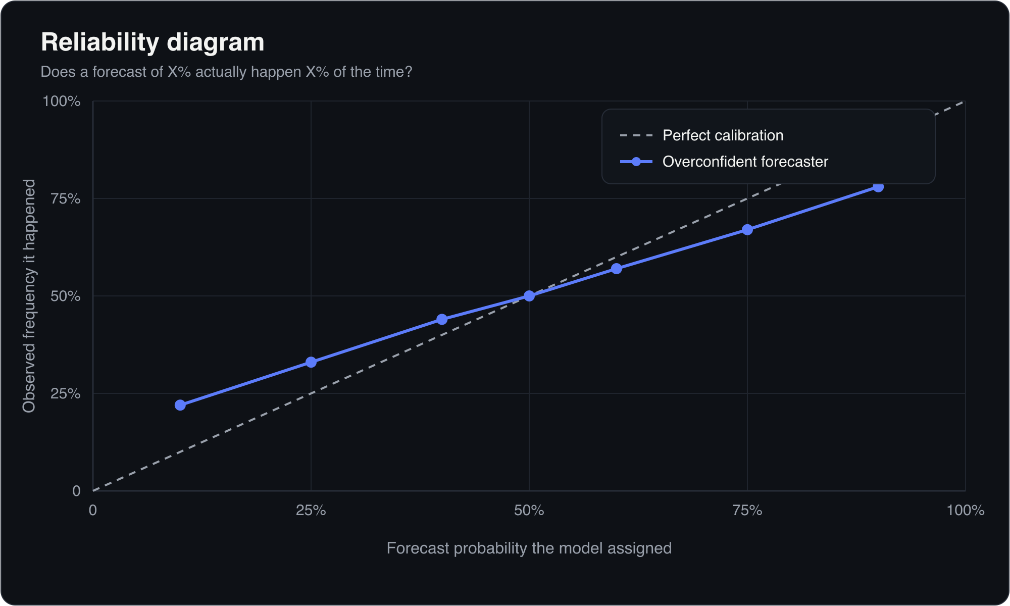
- Perfect calibration is the 45-degree diagonal: when you say 30%, it happens 30% of the time.
- Points below the diagonal mean overconfidence — you said 80% but it only happened 60% of the time.
- Points above the diagonal mean underconfidence — you hedged at 60% when the event happened 80% of the time.
Reliability diagrams visualize exactly the reliability term of the Murphy decomposition (arXiv: Dimitriadis et al.). They are the standard way to show calibration, where the Brier score summarizes it into one number. The two are complementary: the diagram diagnoses the shape of your miscalibration; the score ranks forecasters. Recent statistical work has focused on making these diagrams reproducible and free of arbitrary binning choices (PNAS, 2021).
Brier vs. log loss: choosing a proper scoring rule
Brier is not the only strictly proper scoring rule. The other workhorse is log loss (logarithmic score / cross-entropy):
LL = −(1/N) Σ [ o_t · ln(f_t) + (1 − o_t) · ln(1 − f_t) ]
Both are strictly proper, so both reward honesty. They differ in how harshly they punish confident mistakes (MetricGate):
| Property | Brier score | Log loss |
|---|---|---|
| Penalty shape | Quadratic (squared error) | Logarithmic |
| Range | Bounded, 0 to 1 | Unbounded, 0 to ∞ |
| Confident wrong calls | Capped — worst single error is 1 | Explodes — a 0 on an event that occurs is infinitely penalized |
| Numerical stability | Robust | Fragile; needs probability clipping near 0 and 1 |
| Intuition | ”Mean squared error on probabilities" | "Surprise,” in bits/nats |
The practical trade-off: log loss is the stricter disciplinarian. It savagely punishes overconfidence — assign probability 0 to something that then happens and your score blows up to infinity (MetricGate). That is philosophically appealing (you should never be certain) but operationally brittle, and one freak outcome can dominate an entire evaluation. Brier is gentler and bounded, which makes it more stable for ranking forecasters across many questions and more forgiving of the occasional surprise. Many evaluations, including the 2025 academic study discussed below, report both so neither metric’s blind spot goes unnoticed. The deeper theory of why these rules are “proper” — and how to construct others — is laid out in Gneiting & Raftery (2007), the standard reference.
Tetlock, superforecasting, and why this matters in the real world
The most influential demonstration that calibration is trainable came from the Good Judgment Project (GJP), founded by Philip Tetlock, Barbara Mellers, and Don Moore at the University of Pennsylvania in 2011 (Wikipedia). The GJP competed in a forecasting tournament run by IARPA (the U.S. intelligence community’s research arm) under the Aggregative Contingent Estimation program, answering roughly 100–150 geopolitical questions per year. Every forecast was graded with — what else — the Brier score.
The results reshaped how forecasting is taught. The GJP’s aggregated forecasts were reported to be 35% to 72% more accurate than rival research teams, and IARPA eventually defunded the other teams (Wikipedia). The project also identified a subset of consistently excellent individuals — “superforecasters” — who were reportedly about 30% better than intelligence analysts with access to classified information (AI Impacts summary). (We flag that 30% figure as a widely repeated claim attributed to Tetlock and press coverage rather than a number we can independently audit.) The lesson: the people who win these tournaments are not the boldest callers — they are the best-calibrated ones, and the Brier score is what crowned them.
Prediction markets sit in the same intellectual lineage. The Iowa Electronic Markets were closer to the final outcome than the polls a reported 74% of the time across hundreds of national polls and five U.S. presidential elections from 1988 to 2004 (Berg, Nelson & Rietz, International Journal of Forecasting). But markets are not automatically well-calibrated. A December 2025 study by Joshua Clinton and TzuFeng Huang at Vanderbilt examined ~2,500 markets across Polymarket, Kalshi, and PredictIt in the final five weeks of the 2024 U.S. election, scoring them with log loss and Brier scores, and found materially different accuracy — roughly 67% for Polymarket, 78% for Kalshi, and 93% for PredictIt — alongside evidence of herd-like pricing (DL News). The headline is not the specific percentages — it is that serious analysts reach for Brier and log loss, never win rate, to settle the question.
How MispriceHQ will be graded
This is the standard we hold ourselves to. The MispriceHQ probabilistic model is in development — it has no live track record, has resolved no markets, and we will not pretend otherwise. When it launches, it will be evaluated exactly as this article describes: out-of-sample Brier scores benchmarked against the 0.25 fence-sitter line and against market prices, reported alongside log loss, and published with reliability diagrams so anyone can inspect our calibration rather than take our word for it. A model that cannot beat the market’s own Brier score is not worth trading on, and we intend to show the scorecard either way. Intellectual honesty means publishing the metric that can prove you wrong.
The takeaway for any forecaster, human or model: stop counting wins. Start scoring probabilities. Win rate flatters the overconfident and punishes the honest; the Brier score, decomposed and visualized, tells you the truth about whether your numbers mean what they say.
Frequently asked questions
What is a good Brier score?
Lower is better, on a 0-to-1 scale where 0 is perfect. The key benchmark is 0.25, the score of a 'fence-sitter' who assigns 50% to everything. Any forecaster with genuine information should beat 0.25; a score above it means you are worse than a coin flip. In hard real-world tournaments, scores in the 0.10-0.20 range reflect strong, well-calibrated forecasting. Context matters: easier questions allow lower scores, so always compare against a relevant baseline.
Why is win rate a bad metric for prediction markets?
Win rate only records whether the side you favored happened; it ignores the probability you assigned. A forecaster who says 51% on everything and one who says 99% on everything can have identical win rates while having completely different forecasting skill and risk profiles. On lopsided markets, simply always picking the favorite can post a high win rate with zero real skill. Probabilistic forecasts need a probabilistic metric like the Brier score or log loss.
What is the difference between calibration and accuracy?
Accuracy (win rate) asks whether the outcome landed on the side you leaned toward, treating each forecast as a yes/no call. Calibration asks whether, across all the times you said X%, the event happened X% of the time. A weather forecaster who says '30% rain' and sees rain on exactly 30% of such days is perfectly calibrated, even though it stayed dry most days, something win-rate logic would wrongly penalize. Calibration is the property that matters for probabilities.
Brier score or log loss, which should I use?
Both are strictly proper scoring rules that reward honest probabilities, so neither can be gamed. Brier score is bounded (0 to 1), behaves like mean squared error, and is numerically stable, making it good for ranking forecasters across many questions. Log loss is unbounded and punishes confident errors far more harshly, infinitely penalizing a probability of 0 on an event that occurs. Log loss is stricter but fragile. Many rigorous evaluations report both to cover each metric's blind spots.
What is a reliability diagram?
A reliability diagram (calibration curve) plots your stated probability against the observed frequency of the event. Forecasts are grouped into bins (for example all your 70-80% calls), and each bin shows how often the event actually occurred. Perfect calibration traces the 45-degree diagonal. Points below the line indicate overconfidence; points above indicate underconfidence. It is the standard visual companion to the Brier score, diagnosing the shape of miscalibration that a single number summarizes.
Does MispriceHQ have a working forecasting model?
No. The MispriceHQ probabilistic model is in development. It has no live track record and has resolved no markets, and we will not imply otherwise. When it launches, it will be graded the same way this article describes: out-of-sample Brier scores benchmarked against the 0.25 baseline and against market prices, reported alongside log loss, and published with reliability diagrams so its calibration can be inspected independently rather than taken on trust.
- Brier score — Wikipedia (2026)
- A Brief on Brier Scores — University of Virginia Library (2021)
- Strictly Proper Scoring Rules, Prediction, and Estimation — Journal of the American Statistical Association (Gneiting & Raftery) (2007)
- Brier Score vs Log Loss vs Calibration — MetricGate (2024)
- 1.16. Probability calibration — scikit-learn documentation (2025)
- Evaluating probabilistic classifiers: Reliability diagrams and score decompositions revisited — arXiv (Dimitriadis, Gneiting, Jordan) (2020)
- Stable reliability diagrams for probabilistic classifiers — Proceedings of the National Academy of Sciences (PNAS) (2021)
- The Good Judgment Project — Wikipedia (2026)
- Evidence on good forecasting practices from the Good Judgment Project — AI Impacts (2019)
- Prediction market accuracy in the long run — International Journal of Forecasting (Berg, Nelson & Rietz) (2008)
- Are Polymarket and Kalshi as reliable as they say? Not quite, study warns — DL News (2025-12-05)